Easy LocusZoom-style regional association plot

Creates a regional Manhattan plot focused on a single genomic locus, commonly used for fine-mapping and visualization of association signals with linkage disequilibrium (LD) information. The plot uses genomic coordinate formatting consistent with ez_coverage() and ez_gene(), making it suitable for multi-track visualizations.

Usage

ez_locusZoom(
  input,
  region = NULL,
  gene = NULL,
  gene_db = NULL,
  org_db = NULL,
  extend = 0.1,
  extend_type = c("proportion", "bp"),
  chr = NULL,
  bp = NULL,
  p = NULL,
  snp = NULL,
  logp = TRUE,
  size = 1,
  color = "grey50",
  lead_snp = NULL,
  r2 = NULL,
  colors = NULL,
  highlight_snps = NULL,
  highlight_color = "purple",
  threshold_p = NULL,
  threshold_color = "red",
  threshold_linetype = 2,
  y_axis_style = c("none", "simple", "full"),
  y_axis_label = expression(paste("-log"[10], "(P)")),
  color_by = NULL,
  border = FALSE,
  label_chr = TRUE,
  ...
)

Arguments

input: A data frame containing GWAS results with columns for chromosome, position, p-values, and optionally SNP names. Supports both GWAS-style (CHR, BP, P) and GRanges-style (seqnames, start, pvalue) column naming.
region: Genomic region string (e.g., "chr1:1000000-2000000"). Data is filtered to this region and the x-axis uses coordinate-based formatting. Either region or gene must be provided.
gene: Gene name/symbol to look up (e.g., "PTPRC", "TP53"). When provided, the region is automatically determined from gene coordinates in gene_db. Either region or gene must be provided.
gene_db: TxDb object for gene coordinate lookup when using gene parameter. Required if gene is provided.
org_db: Optional OrgDb object for gene symbol mapping. If NULL (default), auto-detects available OrgDb packages.
extend: Numeric. Amount to extend the region beyond the gene body when using gene parameter. Default: 0.1 (10% of gene length on each side).
extend_type: How to interpret extend: "proportion" (relative to gene length) or "bp" (absolute base pairs). Default: "proportion".
chr: Character string specifying the column name for chromosome numbers. Default: auto-detect from "CHR", "seqnames", "chrom", etc.
bp: Character string specifying the column name for base pair positions. Default: auto-detect from "BP", "start", "pos", etc.
p: Character string specifying the column name for p-values. Default: auto-detect from "P", "pvalue", "p.value", etc.
snp: Character string specifying the column name for SNP identifiers. Default: auto-detect from "SNP", "rsid", "variant_id", etc.
logp: Logical indicating whether to plot -log10(p-values). Default: TRUE.
size: Numeric value for point size in the plot. Default: 1.
color: Default point color when r2 is not provided. Default: "grey50".
lead_snp: Character string or vector of SNP IDs to highlight as the lead variant(s). Highlighted with highlight_color. Default: NULL.
r2: Numeric vector of r² values for coloring points by linkage disequilibrium with lead variant. Must be same length as number of rows in data. When provided, points are colored using a gradient from blue (low LD) to red (high LD). Default: NULL.
colors: Vector of colors for the r² gradient. Default: LocusZoom palette c("blue3", "skyblue", "green2", "orange", "red3").
highlight_snps: Character vector of SNP IDs to highlight, or a data frame with chr, bp, p columns. Default: NULL.
highlight_color: Color for highlighting lead or specified SNPs. Default: "purple".
threshold_p: Numeric p-value threshold for drawing a significance line. If NULL, no line is drawn. Default: NULL.
threshold_color: Color for the significance threshold line. Default: "red".
threshold_linetype: Linetype for the significance threshold line. Default: 2 (dashed).
y_axis_style: Y-axis style: "none", "simple", or "full". Default: "none" (suitable for stacking).
y_axis_label: Label for the y-axis. Default: expression(paste("-log"[10], "(P)")).
color_by: How points should be colored. Can be "r2" (use the r2 argument for LD coloring), "none" (use a single color), or a column name in the data for discrete/continuous coloring. Default: "r2" if r2 is provided, otherwise "none".
border: Logical. If TRUE, adds a black border around the plot panel. Default: FALSE
label_chr: Logical. If TRUE (default), labels the x-axis with the chromosome name (e.g., "Chr1"). Set to FALSE to suppress the x-axis label.
...: Additional arguments passed to geom_manhattan().

Value

A ggplot2 object containing the regional association plot.

Details

This function creates a regional association plot (LocusZoom-style) for GWAS results within a specific genomic region. It supports LD-based coloring, lead SNP highlighting, and is designed to stack with other track types via vstack_plot().

This function is designed for visualizing association results at a single genomic locus, similar to the LocusZoom web tool. Key features:

LD coloring: When r2 is provided, points are colored by linkage disequilibrium with the lead variant, using the classic LocusZoom color scheme (blue → red gradient).
Gene-based regions: Use gene parameter to automatically look up gene coordinates and define the viewing region.
Stackable: Uses scale_x_genome_region() for x-axis formatting, allowing seamless stacking with ez_coverage(), ez_gene(), and other tracks via vstack_plot().

For genome-wide Manhattan plots across multiple chromosomes, use ez_manhattan() instead.

Examples

# Create example data for a region
set.seed(42)
region_data <- data.frame(
  CHR = rep(3, 100),
  BP = seq(1000, 100000, length.out = 100),
  P = c(runif(95, 0.01, 1), runif(5, 1e-8, 1e-4)),
  SNP = paste0("rs", 1:100)
)

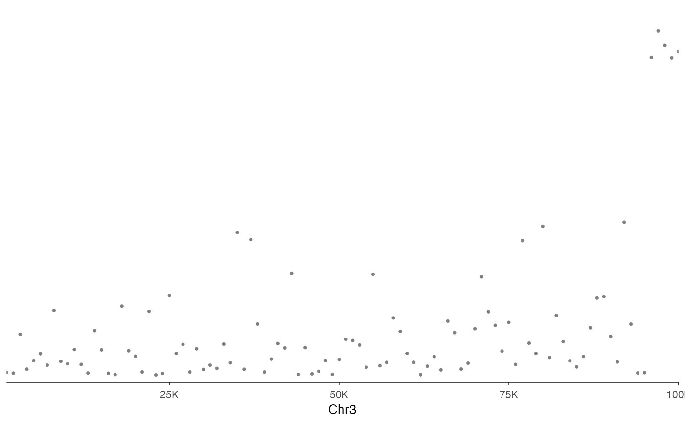
# Basic regional plot
ez_locusZoom(region_data, region = "chr3:1000-100000")


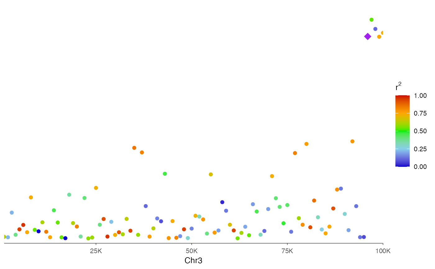
# With LD coloring (simulated r2 values)
# In practice, r2 would come from LD calculations with lead SNP
r2_values <- runif(100, 0, 1)
ez_locusZoom(
  region_data,
  region = "chr3:1000-100000",
  r2 = r2_values,
  lead_snp = "rs96",
  size = 2
)


if (FALSE) { # \dontrun{
# Using gene name to define region (requires TxDb)
library(TxDb.Hsapiens.UCSC.hg38.knownGene)
ez_locusZoom(
  gwas_results,
  gene = "TP53",
  gene_db = TxDb.Hsapiens.UCSC.hg38.knownGene,
  r2 = ld_values
)

# Stack with gene track
p1 <- ez_locusZoom(gwas_results, region = "chr17:7500000-7700000", r2 = ld)
p2 <- ez_gene(txdb, region = "chr17:7500000-7700000")
vstack_plot(p1, p2, heights = c(2, 1))
} # }

Usage

Arguments

Value

Details

See also

Examples