tracks_sashimi

library(ezGenomeTracks)
#> Warning: replacing previous import 'AnnotationDbi::select' by 'dplyr::select'
#> when loading 'ezGenomeTracks'
#> ezGenomeTracks v0.0.1
#> Easy and flexible genomic track visualization
#> Use citation('ezGenomeTracks') to see how to cite this package
#> For documentation and examples, visit: https://github.com/zmu/ezGenomeTracks

Sashimi plots are an elegant way to visualize mRNA splicing data, but few existing tools can do it. Years ago I wrote a custom track class for pyGenomeTracks and have seen several people using it. Here, ezGenomeTracks provides a unified ez_sashimi function that makes it even easier to plot Sashimi plots. It takes a bigwig file and a link file as inputs.

bw0 <- system.file(
  "extdata",
  "avg_chr2-231091223_231109786_231113600_0.bw",
  package = "ezGenomeTracks"
)

bw1 <- system.file(
  "extdata",
  "avg_chr2-231091223_231109786_231113600_1.bw",
  package = "ezGenomeTracks"
)

bw2 <- system.file(
  "extdata",
  "avg_chr2-231091223_231109786_231113600_2.bw",
  package = "ezGenomeTracks"
)

link0 <- data.table::fread(
  system.file(
    "extdata",
    "chr2-231091223_231109786_231113600_0.sashimi",
    package = "ezGenomeTracks"
  ),
  header = F,
  col.names = c("seqnames", "start", "end", "name", "score", "strand")
)

link1 <- data.table::fread(
  system.file(
    "extdata",
    "chr2-231091223_231109786_231113600_1.sashimi",
    package = "ezGenomeTracks"
  ),
  header = F,
  col.names = c("seqnames", "start", "end", "name", "score", "strand")
)

link2 <- data.table::fread(
  system.file(
    "extdata",
    "chr2-231091223_231109786_231113600_2.sashimi",
    package = "ezGenomeTracks"
  ),
  header = F,
  col.names = c("seqnames", "start", "end", "name", "score", "strand")
)

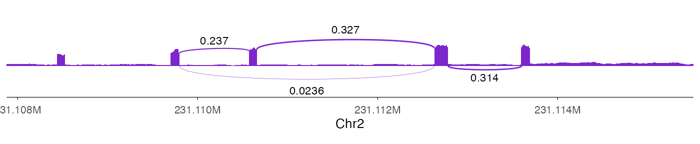
head(link0)
#>    seqnames     start       end   name      score strand
#>      <char>     <int>     <int> <char>      <num> <char>
#> 1:     chr2 231109795 231110578  link1 0.23729710      +
#> 2:     chr2 231109795 231112631  link2 0.02362313      +
#> 3:     chr2 231110655 231112631  link3 0.32665704      +
#> 4:     chr2 231112780 231113600  link4 0.31368420      +

ez_sashimi(
  coverage_data = bw0,
  junction_data = link0 |> dplyr::mutate(score = signif(score, 3)),
  linewidth_range = c(0.1, 0.5),
  height_factor = 0.03,
  region = "chr2:231107879-231115507",
  junction_curvature = 0.03
)

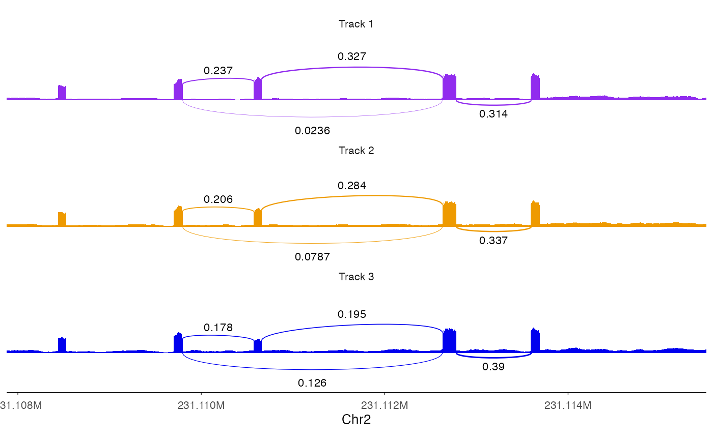
We can plot multiple track together as we do for ez_coverage.

ez_sashimi(
  coverage_data = list(bw0, bw1, bw2),
  junction_data = list(
    link0 |> dplyr::mutate(score = signif(score, 3)),
    link1 |> dplyr::mutate(score = signif(score, 3)),
    link2 |> dplyr::mutate(score = signif(score, 3))
  ),
  linewidth_range = c(0.1, 0.5),
  height_factor = 0.03,
  region = "chr2:231107879-231115507",
  junction_curvature = 0.03,
  colors = c("purple2", "orange2", "blue2")
)