library(ezGenomeTracks)
#> Warning: replacing previous import 'AnnotationDbi::select' by 'dplyr::select'
#> when loading 'ezGenomeTracks'
#> ezGenomeTracks v0.0.13
#> Easy and flexible genomic track visualization
#> Use citation('ezGenomeTracks') to see how to cite this package
#> For documentation and examples, visit: https://github.com/zmu/ezGenomeTracks
ezGenomeTracks provides two specialized functions for
visualizing GWAS association data:
-
ez_manhattan()- Genome-wide Manhattan plots across multiple chromosomes -
ez_locusZoom()- Regional association plots (LocusZoom-style) for a single locus
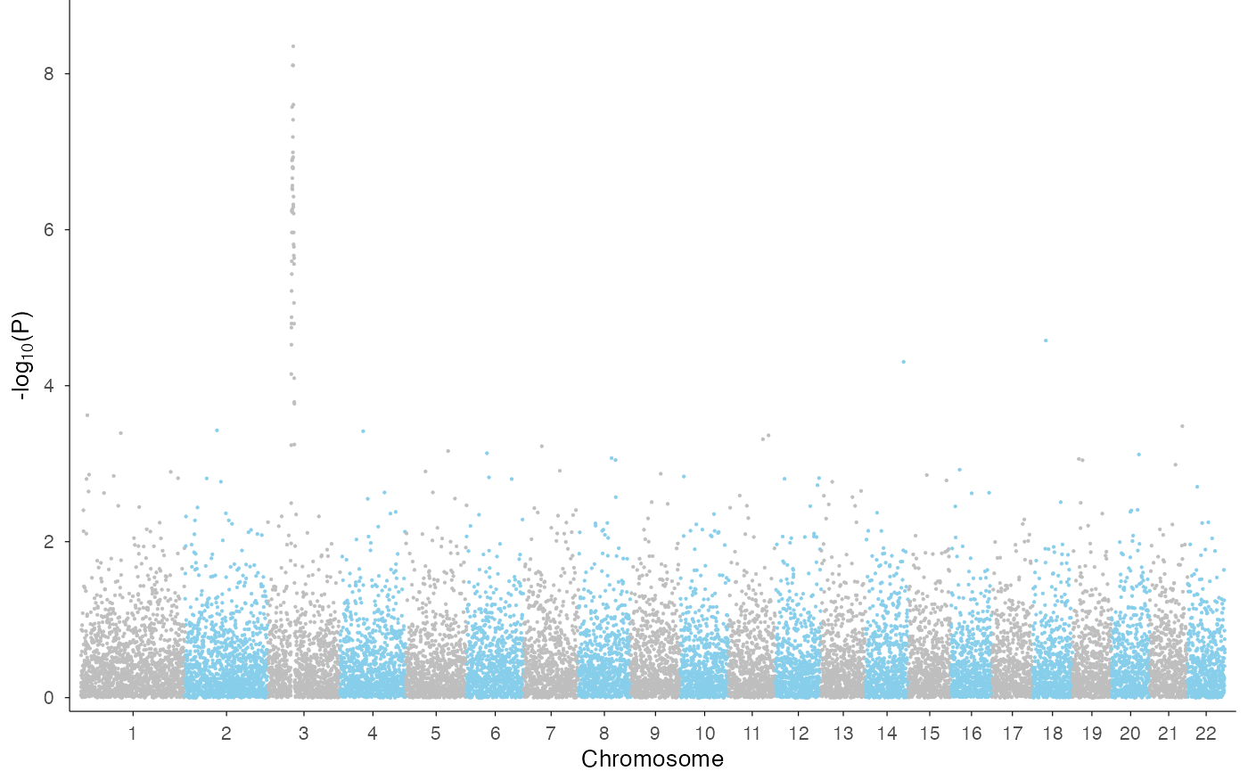
Genome-wide Manhattan plot
Use ez_manhattan() to visualize GWAS results across the
entire genome. We use the example GWAS data from qqman
package to demonstrate.
library(qqman)
#>
#> For example usage please run: vignette('qqman')
#>
#> Citation appreciated but not required:
#> Turner, (2018). qqman: an R package for visualizing GWAS results using Q-Q and manhattan plots. Journal of Open Source Software, 3(25), 731, https://doi.org/10.21105/joss.00731.
#>
head(gwasResults)
#>   SNP CHR BP         P
#> 1 rs1   1  1 0.9148060
#> 2 rs2   1  2 0.9370754
#> 3 rs3   1  3 0.2861395
#> 4 rs4   1  4 0.8304476
#> 5 rs5   1  5 0.6417455
#> 6 rs6   1  6 0.5190959
ez_manhattan(
  input = gwasResults,
  chr = "CHR",
  bp = "BP",
  p = "P",
  colors = c("grey", "skyblue")
)
You can add a genome-wide significance threshold line:
ez_manhattan(
  input = gwasResults,
  chr = "CHR",
  bp = "BP",
  p = "P",
  colors = c("grey", "skyblue"),
  threshold_p = 5e-8,
  threshold_color = "red"
)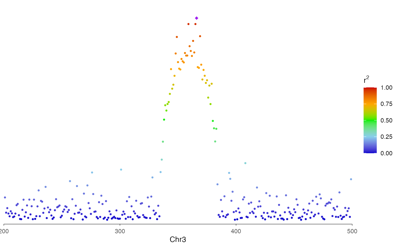
Regional association plot (LocusZoom-style)
Use ez_locusZoom() to create regional association plots
focused on a single locus. This is ideal for fine-mapping visualization
and can be stacked with other genomic tracks.
# Filter data to a specific region
region <- "chr3:200-500"
locusResults <- gwasResults |>
  dplyr::filter(CHR == 3 & BP > 200 & BP < 500)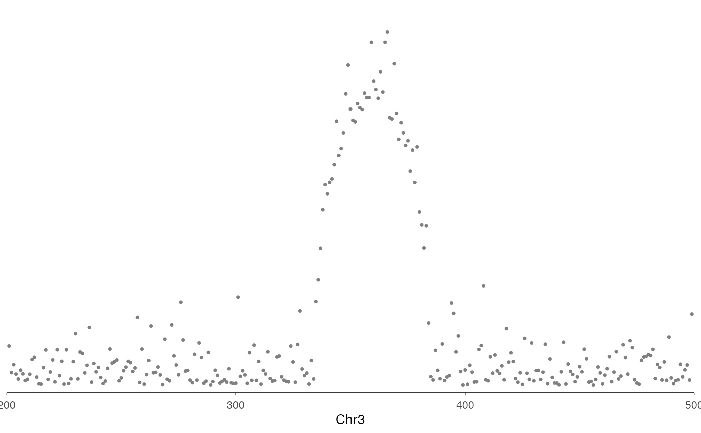
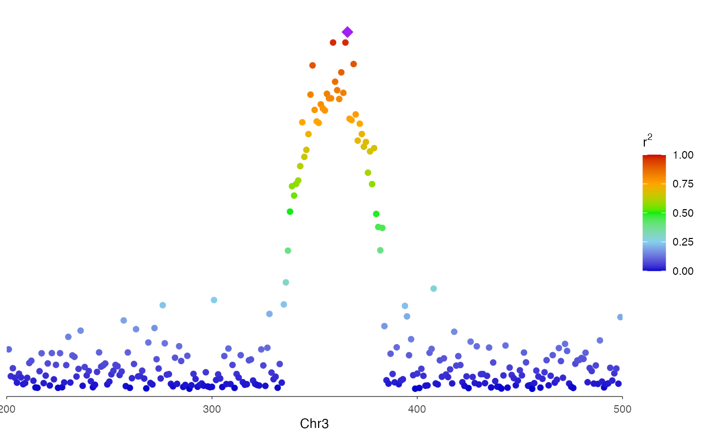
With LD coloring
You can use the r2 option to color the dots by linkage
disequilibrium with a lead variant. This creates the classic LocusZoom
color gradient. For demonstration purpose, here we use p-value to create
a continuous color for r2.
# Simulated r2 values (in practice, these come from LD calculations)
r2_values <- -log10(locusResults$P) / max(-log10(locusResults$P))

ez_locusZoom(
  input = locusResults,
  region = region,
  snp = "SNP",
  lead_snp = "rs3057",
  r2 = r2_values,
  size = 2
)